Tuesday, October 27, 2015

Industrial Instrumentation Mini Project

Industrial Instrumentation Mini Project

Both Thermistors and RTD’s are basically resistors whose resistance varies with temperature.

Thermistors differ from resistance temperature detectors (RTDs) in that the material used in a thermistor is generally a ceramic or polymer, while RTDs use pure metals. The temperature response is also different; RTDs are useful over larger temperature ranges, while thermistors typically achieve a greater precision within a limited temperature range, typically −90 °C to 130 °C.

linearization using parallel resistance

Parallel connection of resistance to thermistor

So we have high sensitivity and fast response in favor of thermistor, but the non linear behavior is a drawback that we must try to correct.
In tackling this problem the basic approach can be to connect a parallel resistor to the thermistor.
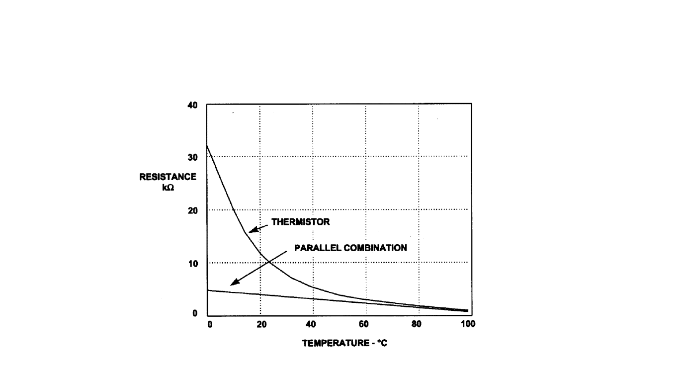
Linearization by connecting a resistance in parallel

But as you can see above even though this improves the resistance - temperature relationship in terms of linearity, the sensitivity of the thermistor is sacrificed.

Temperature to Period Linearization technique

We will be using a circuit (shown below which functions as a relaxation oscillator) to get a linear relationship between our input variable (Temperature) and output variable (in this circuit it’s the time period).
It is important to note the importance of linearization, we have useful tools used in systems analysis which are applicable to linear systems.
So as it’s much easier to deal mathematically with linear relationships when compared to non linear systems.

Here the output will be a periodic waveform with a time period , here this output waveforms time period is the output variable which is linearised w.r.t. to temperature, unlike the thermistor’s resistance which is non linear w.r.t. to temperature.

Nonlinear behavior of thermistor resistance wrt temprature

Theoretical modeling of T - R characteristics

Now for the modeling of the relationship between the temperature and resistance for the thermistor we can use first order approximation, but this approximation involves assumptions such as carrier mobility’s invariance with temperature etc which are not valid across the entire operating range of the temperature.

Note that for a even more accurate description of the thermistor we use third order approximations like the Steinhart–Hart equation and Becker-Green-Pearson Law which has 3 constants.
Even the original Bosson’s law has 3 constants and is written as

This is approximated to the second order law,

In the above formula’s are constants and stands for temperature while stands for thermistor resistance.

The reason why we go for the 2 constant law rather than the 3 constant law even though the third order approximation fits better is that comparatively its harder to use hardware linearization techniques.1
Also this relationship closely represents an actual thermistor’s behavior over a narrow temperature range.

So if we are going for third order approximations we should use take advantage of the advancements in computing and just obtain a analog voltage proportional to the thermistor resistance, then use ADC to get the digital values which can simply be fed into the 3rd order equation.

Working of the circuit

Circuit Diagram for linearization of thermistor output

We should observe the non linearity error is within 0.1K over a range of 30K for this linearization circuit.

Read more from what S.Kaliyugavaradan has written.

References

Written with StackEdit.


  1. Wiley Survey of Instrumentation and Measurement, by Stephen A. Dyer published by John Wiley & Sons. Page 126
    Read here

Wednesday, October 7, 2015

Homomorphic filtering

Prerequisites : Basics of Fourier Transform, High pass filters in the context of Image processing.

I will be talking about this filtering method in terms of using it as an enhancement technique, but it can be leveraged for other uses also.

The Wikipedia Page and this blog explains this entire concept thoroughly.

First let me start with the illumination-reflectance model of image formation which says that the intensity of any pixel in an image (which is the amount of light reflected by a point on the object and captured by an imaging system) is the product of the illumination of the scene and the reflectance of the object(s) in the scene.

where is the image, is scene illumination, and is the scene reflectance. Reflectance arises from the properties of the scene objects themselves, but illumination results from the lighting conditions at the time of image capture.

This model should make sense because reflectance is basically the ratio of light reflected to the light received (illumination). But in case you are still not feeling like this equation makes sense then consider this image.

Golf ball

Here the image is the collection of values that tell us the intensity of light reflected from each point. For example the golf ball reflects more light, while the hole reflects less. These values form a matrix in the shape of the image - .

Now what causes the golf ball to reflect more light than the grass? it’s a property of the material which decides what wavelengths of light are reflected and which are absorbed. We call a measure of this property as reflectance and the matrix holds that value for all these points.

The imaging system - our camera, captures the light reflected from each point which is the product of the illumination hitting each point with the “reflectance” property of the material at these respective points.

So what we want is actually only that property - which will be faithfully reflected in the image matrix if the illumination on the objects are uniform. In the case we hide the golf ball under a shadow while shining light on the grass, the image will turn out to show the golf ball as not as white as it actually is.

Golf ball in the shade

Now in such images taken in non-uniform illumination setting, Illumination typically varies slowly across the image as compared to reflectance which can change quite abruptly at object edges.

If the light source is placed at such a position that it regularly illuminates the scene then we won’t have the problem of irregular illumination, but consider it being placed in a direction such that part of the scene is highly illuminated, while the remaining part of the scene is in the shadows. Now it should be obvious that due to the properties of light, the 2 areas are separated by fuzzy area where it’s not fully illuminated nor is it in the shadows. This is what I mean by the Illumination typically varies slowly across the image . For example check out the photo at the bottom of the post.

But objects stand out among the background because at the object edges the intensity of light reflected (as compared to the background) changes abruptly, as you can see the black text has a high contrast with the white background.

So as far as the image is concerned, the uneven illumination - is the noise (Multiplicative noise - because is multiplied to ) that we wish to remove. Because the illumination term is what causes part of the scene to be in the shadows, and is the signal that we need - it holds the information about everything ‘s visual properties (how much a particular point absorbs/reflects light)

In order to make this removal easy we shift the domain of the image from the spatial domain of to the domain - . Here,


The property’s of log makes the image such that these multiplicative components can be separated linearly in the frequency domain.

Illumination variations can be thought of as a multiplicative noise in the spatial domain while its linear noise in the log domain.

Now the question comes why linear, the point is that we need to be able to separate and , so that we can remove without harming

As we can see the Fourier transform - of the image (shifting it from spatial domain - to the frequency domain - ) does not separate the illumination and reflectance components. Rather the multiplicative components become convolved in the frequency domain as per the Convolution theorem.

But the log of the spatial domain - when shifted to frequency domain lets us express the the image (now ) as the linear sum of and because the fourier transform is linear.


Now that separability has been achieved, we can apply high pass filtering to ,

So as will have energy compaction among low frequency components, while will have the same for high frequency components. We can see that the term will become attenuated to a great degree (Depending on the filter and the cutoff frequency set).

so we will have

So now after the high pass filtering of the fourier of the log of actual image (Whew that was a stretch! lol)

we see that we get the fourier of the log of the reflectance component of the image - , and that was what we were trying to isolate all along.

so to get the reflectance back in the spatial domain we take the exponential of the inverse fourier transform of , so we get a close approximation to - .

To clarify why we do exponential and inverse fourier transform (IFT), we are just backtracking to the spatial domain, we are doing IFT to get back to the log of the spatial domain - . And then depending on the base we use to get the log domain (I assumed natural logarithm so I said exponential), if you use base 10, then we need to do to the power 10 in order to get back to (x,y).

And so we have successfully filtered out the multiplicative noise that is the slowly varying illumination - from the image - .

I got the code from the blog post I mentioned at the top of the post. My modifications were minor, I just added a line to convert the image to grayscale in case you wanted to operate homomorphic filtering on a color image.

and the results when I ran it on a irregularly illuminated image was pretty awesome - Output of homomorphic filtering with HPF

I know it’s tough to argue that the right image is enhanced visually w.r.t human eyesight, but as you can see the “irregular illumination” has disappeared. This shows us how homomorphic filtering is just another tool in our toolbox and has its own use cases.

Written with StackEdit.

Matrix Chain Multiplication

We got a assignment problem from our IC 303 DATA STRUCTURES AND ALGORITHMS , I’ll be going into its portions in detail too. But for today’s post I will solve the following problem of Matrix Chain Multiplication and hope the explanation of this problem will help bring clarity to how useful dynamic problem can be in solving problems.

The Assignment Problem

Find the cost involved in finding the product of 6 Matrices using both

  1. Dynamic programming (Matrix Chain Multiplication)
  2. Normal matrix multiplication.

Given,

Now first of all, what is cost here? I think its reasonable to assume the cost (time complexity) can be thought of as the total number of scalar multiplications to obtain .

For calculating given that,

its trivial to prove that the number of scalar multiplications required are .

For each element of we need to do multiplications, for the first row of we have such elements(size of each row), so multiplications.

Finally we have such rows (number of rows), so total number of scalar multiplications to calculate is

For example check out the image below where are 4,2,3.

Matrix Multiplication

Normal matrix multiplication.

Ok, now we have defined what is cost let’s see what the cost of the Normal Multiplication of the The Assignment problem is,

now by normal multiplication lets consider the grouping as shown below,

So here first is done in
then that solution with is done in

Thus in the Normal method we need to perform scalar multiplications.

Now it should be obvious we can find by different methods which will change as we change how we group the 6 matrices.

Therefore the matrix-chain multiplication problem is given a chain of matrices to multiply, we need to find the grouping which minimizes the total number of scalar multiplications

In most cases the time we spend to find this special grouping is more than made up by the savings in the effort to actually compute the solution.

Now ok cool, we now know that we need to group these matrices, what’s the total number of ways that can be done?

Going by brute force then using the native algorithm the time complexity is,

while we get for the dynamic programming solution to finding the grouping.

So we can agree we need to use dynamic programming to optimally parenthesize a matrix chain.

Dynamic programming

I hope you all know that Divide and conquer algorithms works on the principle that we take a problem, make it into subproblems (divide) and recursively solve it (conquer).

Now what if when you applied this kind of problem solving strategy to a problem and discovered that you were repeating your work. That the subproblems that you were solving weren’t unique… would you solve them again and again? Nope, we would use the solution we already got with the first occurrence of that particular subproblem right?!

So that’s the basic idea of how Dynamic programming works. So when we see a problem with both Overlapping subproblems (this means that the subproblems repeat themselves) and Optimal substructure (which just means that it’s possible to solve this problem optimally by joining the optimally solved subproblems) we can use D.P.

So in the case of this Matrix Chain Multiplication problem what’s this “optimal subproblem” look like?

The crucial idea is that given a set of matrices then the Matrix Chain Multiplication problem can be broken down to,
Finding ( ) such that both the group of matrices to as well as the group of matrices to are optimally arranged for multiplication.

Thus

where p is the number of rows of the first matrix,
q is the number of rows of th matrix
or the number of column of th matrix,
r is the number of columns of the th matrix.

So here the first two terms are the cost of optimally solving the subproblems (i.e. consider the set of matrices and as subproblems) now when you join those two subproblem solutions you get the optimal solution to the original problem involving . That’s the key idea here.

Optimal solution of =
The term is incurred by the joining of the two subproblem solutions. (the first solution is a matrix and the second solution is a matrix.)

[TO BE CONTINUED]

Written with StackEdit.